Hands-On Lab: Conditional Formatting Without IF

Welcome to the Hands-On Lab (HOL) session with TTC! On this page, we'll learn how to use Conditional Formatting in Excel—without relying on IF formulas. This technique is perfect for making your data more interactive and visually appealing with just a few clicks and simple logic.

Many Excel users tend to use IF for conditional coloring, but there's a more efficient way by applying logical operators directly via the Conditional Formatting menu. This tutorial will walk you through a real-world example that you can follow right away.

Let’s start practicing and prove that beautifying Excel data doesn’t have to be complicated!

🧩 Case Study

You have a score table like this:

    | Name | Score |
    |------|-------|
    | Asep | 60    |
    | Budi | 59    |
    | Cici | 45    |
    | Dedi | 30    |
    

The goal: automatically color the Score column:

• Score < 60: Light red (Needs remedial)
• Score ≥ 60: Light green (Pass)

✨ Step-by-Step

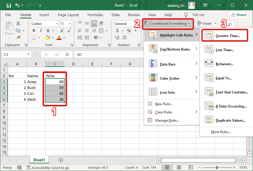
1. Select the score column, e.g., cells C3:C6.
2. Go to Home → Conditional Formatting → Highlight Cells Rules.
3. Choose the "Greater Than..." option.
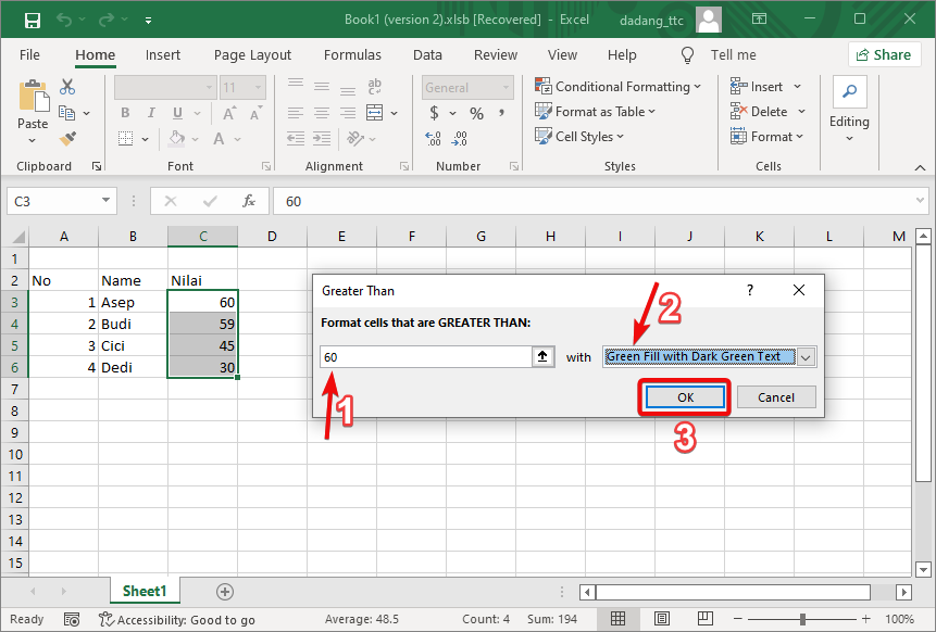
4. Enter the value without using IF, for example:

   60

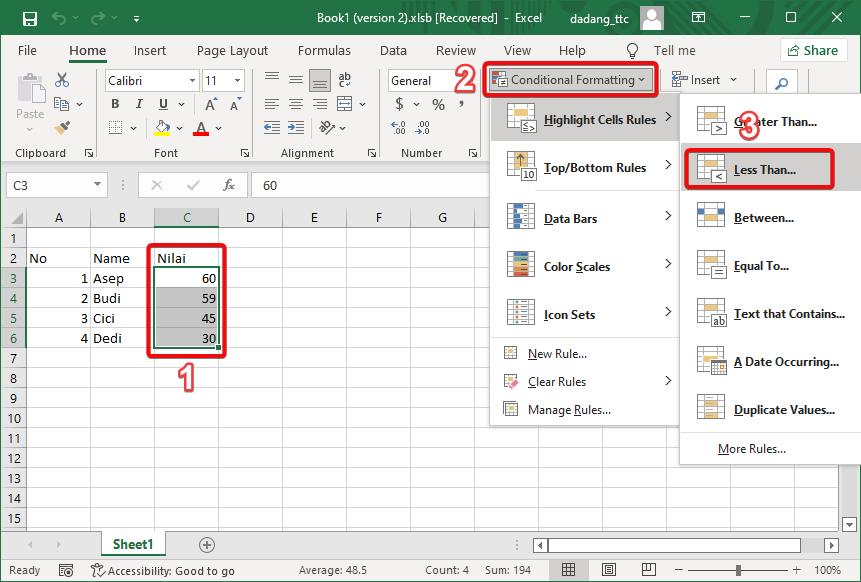
   then choose the format Green Fill with Dark Green Text.
5. Repeat step 2 for the "fail" condition:

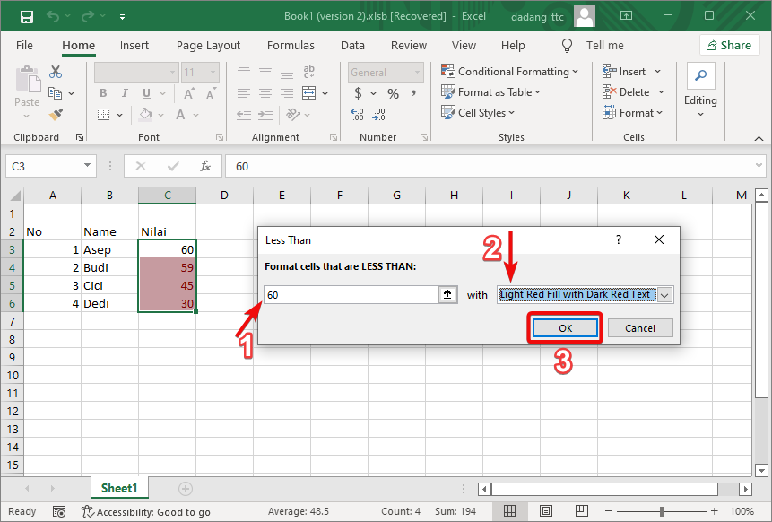
   60

   using the format Light Red Fill with Dark Red Text.

💡 Key Notes

• Use direct logical rules without the IF() formula.
• Excel will treat B2 as the starting cell and apply formatting downward.
• This technique is cleaner and renders faster in Excel.