Hands-On Lab: Conditional Formatting Without IF

Welcome to the Hands-On Lab (HOL) session with TTC! On this page, you will learn how to use Conditional Formatting in Excel without relying on IF formulas. This technique is ideal for creating visually clear and interactive data using only a few clicks and simple logic.

Many Excel users depend on IF formulas for conditional coloring, even though there is a more efficient approach using logical operators directly within the Conditional Formatting menu. This tutorial will guide you step by step through real-world examples that you can practice immediately.

Let’s start practicing and prove that beautifying Excel data doesn’t have to be complicated!

📊 Dataset Used

Throughout this Conditional Formatting tutorial series, we use a single main dataset in the form of a student score list with the following characteristics:

• Number of students: 15
• Classes: A and B
• Subjects: Religion, Science, Social Studies, Indonesian Language, Sports
• Score range: 55 – 90

This dataset was intentionally selected because it contains high, medium, and low values, making it ideal for practicing various types of Conditional Formatting without IF formulas.

🧩 Initial Case Study (Simple Example)

Before working with the full dataset, we start with a simple example to understand the basic concept of automatic formatting using Highlight Cells Rules.

You have a score table like this:

    | Name | Score |
    |------|-------|
    | Asep | 60    |
    | Budi | 59    |
    | Cici | 45    |
    | Dedi | 30    |
      

Objective: automatically apply color formatting to the Score column:

• Score < 60: Light red (Needs remedial)
• Score ≥ 60: Light green (Pass)

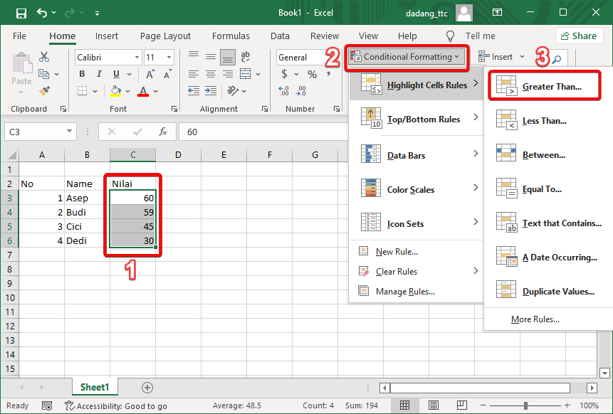
✨ Step-by-Step

1. Select the score column, for example cells C3:C6.
2. Go to Home → Conditional Formatting → Highlight Cells Rules.
3. Select the "Greater Than..." option.
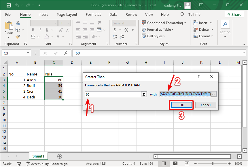
4. Enter the value without using IF:

   60

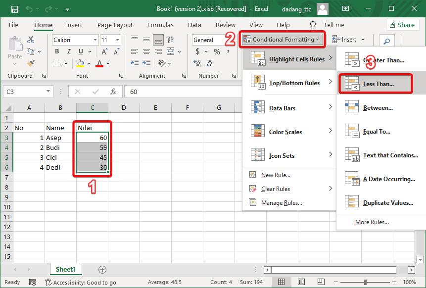
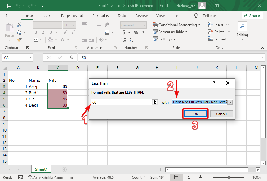
   then choose Green Fill with Dark Green Text.
5. Repeat step 2 for the failing condition:

   60

   using Light Red Fill with Dark Red Text.

💡 Important Notes

• Use direct logical rules without the IF() formula.
• Excel treats the first selected cell as the reference and applies formatting downward automatically.
• This method is cleaner and renders faster in Excel.

🧭 Types of Conditional Formatting Covered

• Highlight Cells Rules
  Used to highlight values based on specific conditions (for example: pass or remedial). (Video available)

🎥 Video Tutorial: Highlight Cells Rules

• Top / Bottom Rules ✅
  Automatically highlights the highest or lowest values (example: Top 3 Science scores or Bottom 5 Social Studies scores). (Video available)

🎥 Video Tutorial: Top & Bottom Rules

• Data Bars, Color Scales & Icon Sets
  Visualize data using bars, color gradients, and icon indicators to quickly identify patterns and trends. (Video available)

🎥 Video Tutorial: Data Bar, Color Scale & Icon Sets

All of these features are applied using the same dataset, allowing you to visually compare the results of each formatting approach.

📌 Summary

Conditional Formatting allows us to interpret Excel data visually without lengthy IF logic. Using a single dataset, we can clearly see the differences and benefits of each formatting rule type.